# import basics
import matplotlib as mpl
import matplotlib.pyplot as plt
import numpy as np

# import pyathena 
import sys
sys.path.insert(0,'../../')
import pyathena as pa

---------------------------------------------------------------------------
ModuleNotFoundError                       Traceback (most recent call last)
Cell In[1], line 9
      7 import sys
      8 sys.path.insert(0,'../../')
----> 9 import pyathena as pa

File ~/work/pyathena-1/pyathena-1/docs/examples/../../pyathena/__init__.py:42
      3 # __all__ is taken to be the list of module names that should be imported when
      4 # from `package import *` is encountered
      5 # https://docs.python.org/3/tutorial/modules.html#importing-from-a-package
      7 __all__ = [
      8            # Units class
      9            "Units",
   (...)
     39            "LoadSimCoreFormationAll",
     40            ]
---> 42 from .io.read_vtk import read_vtk, AthenaDataSet
     43 from .io.read_athinput import read_athinput
     44 from .io.read_hst import read_hst

File ~/work/pyathena-1/pyathena-1/docs/examples/../../pyathena/io/read_vtk.py:17
     13 import astropy.units as au
     15 from .athena_read import vtk
---> 17 from ..util.units import Units
     19 def read_vtk_athenapp(filenames):
     20     x1f = []

File ~/work/pyathena-1/pyathena-1/docs/examples/../../pyathena/util/__init__.py:4
      2 from .units import Units, ac, au
      3 from .rebin import rebin_xyz, rebin_xy
----> 4 from .mass_to_lum import mass_to_lum
      5 from .piecewisepowerlaw import PiecewisePowerlaw
      6 from .sb99 import SB99

File ~/work/pyathena-1/pyathena-1/docs/examples/../../pyathena/util/mass_to_lum.py:4
      1 from __future__ import print_function
      3 import numpy as np
----> 4 from scipy.interpolate import interp1d
      6 from .piecewisepowerlaw import PiecewisePowerlaw
      8 class mass_to_lum(object):

ModuleNotFoundError: No module named 'scipy'

Cooling in TIGRESS-classic

See Figure 1 in Kim and Ostriker [2017]

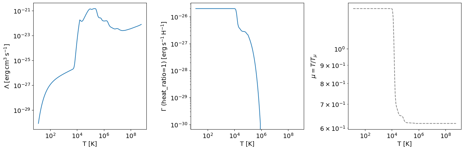
Tabulated cooling/heating coefficients

• Original form is taken from Koyama & Inutsuka (2004; with typo correction in Kim et al. (2008)) at \(T<10^{4.2}{\rm K}\) and Sutherland & Dopita (1993) for \(T>10^{4.2}{\rm K}\)

• Volumetric cooling/heating rates are: \(n_{\rm H}^2\Lambda(T)\) and \(n_{\rm H}\Gamma\). \(\Gamma\) is proportional to the heat_ratio field in the code (unity for the solar neighborhood condition)

• Pressure, mean molecular weight, temperature, electron abundance, etc.

  \[ P = \dfrac{\rho k_{\rm B}T}{\mu m_{\rm H}} = \dfrac{\rho k_{\rm B}T_{\mu}}{m_{\rm H}}= \dfrac{n_{\rm H}k_{\rm B}T}{\mu_{\rm H}m_{\rm H}} \approx (n_{\rm H^0} + n_{\rm H^+} + n_{\rm H_2} + n_{\rm He} + n_{\rm e}) k_{\rm B}T \approx (1.1 + x_{\rm e} - x_{\rm H_2})n_{\rm H}k_{\rm B}T \]

  where \(T_{\mu} \equiv T/\mu\), \(x_{\rm e} = n_{\rm e}/n_{\rm H}\), and \(x_{\rm H_2} = n_{\rm H_2}/n_{\rm H}\), and so on.

• The quantity \(T_{\mu} \propto P/n_{\rm H}\) is easy to evolve in the cooling module.

• In the TIGRESS-classic cooling function,

  • \(\mu_H = \rho/(n_{\rm H}m_{\rm H}) = 1.4271\)

  • \(x_{\rm H_2} = 0\).

  • \(T\), \(\Lambda(T)\), \(\Gamma(T)\) are tabulated as functions of \(T_\mu\) (or the T1 field in the code)

cf = pa.classic.coolftn
c = cf.get_cool(cf.T1)
h = cf.get_heat(cf.T1)
T = cf.get_temp(cf.T1)

mpl.rcParams['font.size'] = 14
fig, axes = plt.subplots(1, 3, figsize=(15,5))
plt.sca(axes[0])
plt.loglog(T, c)
plt.xlabel('T [K]')
plt.ylabel(r'$\Lambda\;[{\rm erg}\,{\rm cm}^{3}\,{\rm s}^{-1}]$')

plt.sca(axes[1])
plt.loglog(T, h)
plt.xlabel('T [K]')
plt.ylabel(r'$\Gamma$ (heat_ratio=1) $[{\rm erg}\,{\rm s}^{-1}\,{\rm H}^{-1}]$')
plt.tight_layout()

plt.sca(axes[2])
plt.loglog(T, T/cf.T1, 'grey', ls='--')
plt.xlabel('T [K]')
plt.ylabel(r'$\mu = T/T_{\mu}$')
plt.tight_layout()

u = pa.Units()
print(u.muH)
nH_eq = h/c
# 1.1 + xe = u.muH/(temp/cf.T1)
pok_eq = nH_eq*u.muH*cf.T1
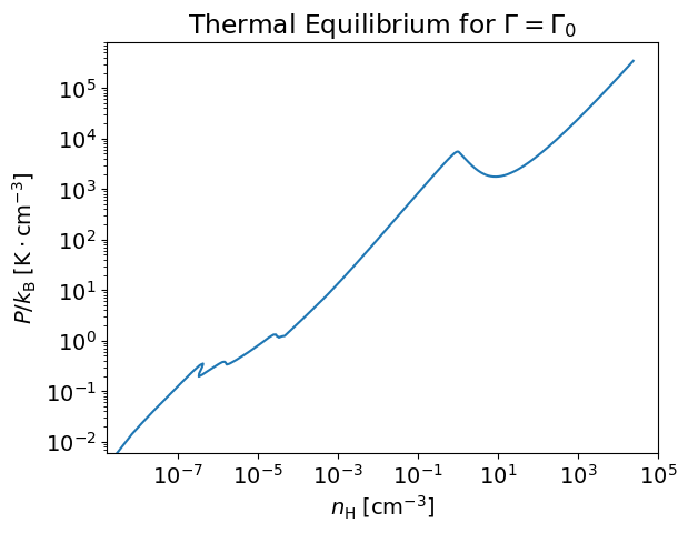
plt.loglog(nH_eq,pok_eq)
plt.xlabel(r'$n_{\rm H}\;[{\rm cm}^{-3}]$')
plt.ylabel(r'$P/k_{\rm B}\;[{\rm K}\cdot{\rm cm}^{-3}]$')
plt.title(r"Thermal Equilibrium for $\Gamma=\Gamma_0$")
# plt.xlim(1e-3,1e5)
# plt.ylim(1e1,1e6)

1.4271

Text(0.5, 1.0, 'Thermal Equilibrium for $\\Gamma=\\Gamma_0$')